Networks (experimental)

Using the feature

Step-by-step workflow — enable, prepare inputs, choose an engine, run, read the output, and price the network.

A practical walkthrough for running Networks mode in QGIS.

Experimental feature. Networks mode is under active development. Some technical aspects are still being validated with domain researchers. If you find results that don’t make sense, please open a GitHub issue or email co2gis.support@gmail.com.

1. Enable experimental network mode

Open the plugin Settings dialog and tick the network-mode checkbox. The setting persists across QGIS restarts. Reload the plugin for the UI to pick it up.

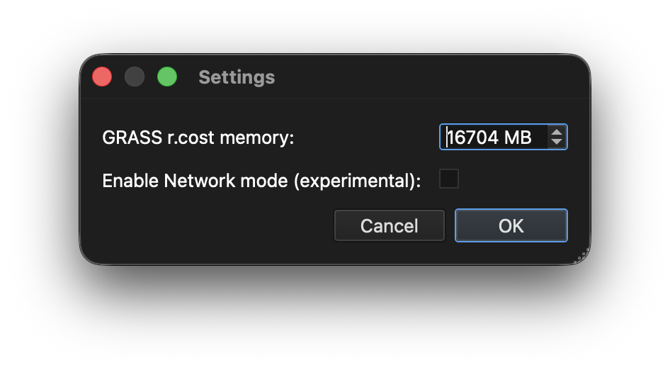
Settings dialog — tick "Enable Network mode (experimental)" and set GRASS r.cost memory

Once enabled, the LCP tab gains a Single / Network mode selector. The run button is labelled “Create Network (experimental)“.

2. Prepare the inputs

Build the combined COMET cost raster first using the earlier tabs (Land Use, Slope, Corridors, Crossings) — this is the same surface used by the single-route tool.

You also need two point layers:

a sources layer (CO₂ emitters), with a numeric attribute for each source’s flow in Mt/yr;
a sinks layer (storage/injection sites), with a numeric attribute for each sink’s injection capacity in Mt/yr.

All layers must be in a projected metric CRS (see the CRS requirement in Sample data). Points are reprojected to the raster’s CRS automatically if needed.

3. Choose the engine

In the Network page, select an Optimisation method:

Heuristic (fast) — always available, no extra dependencies. Connects every source. No additional inputs required.

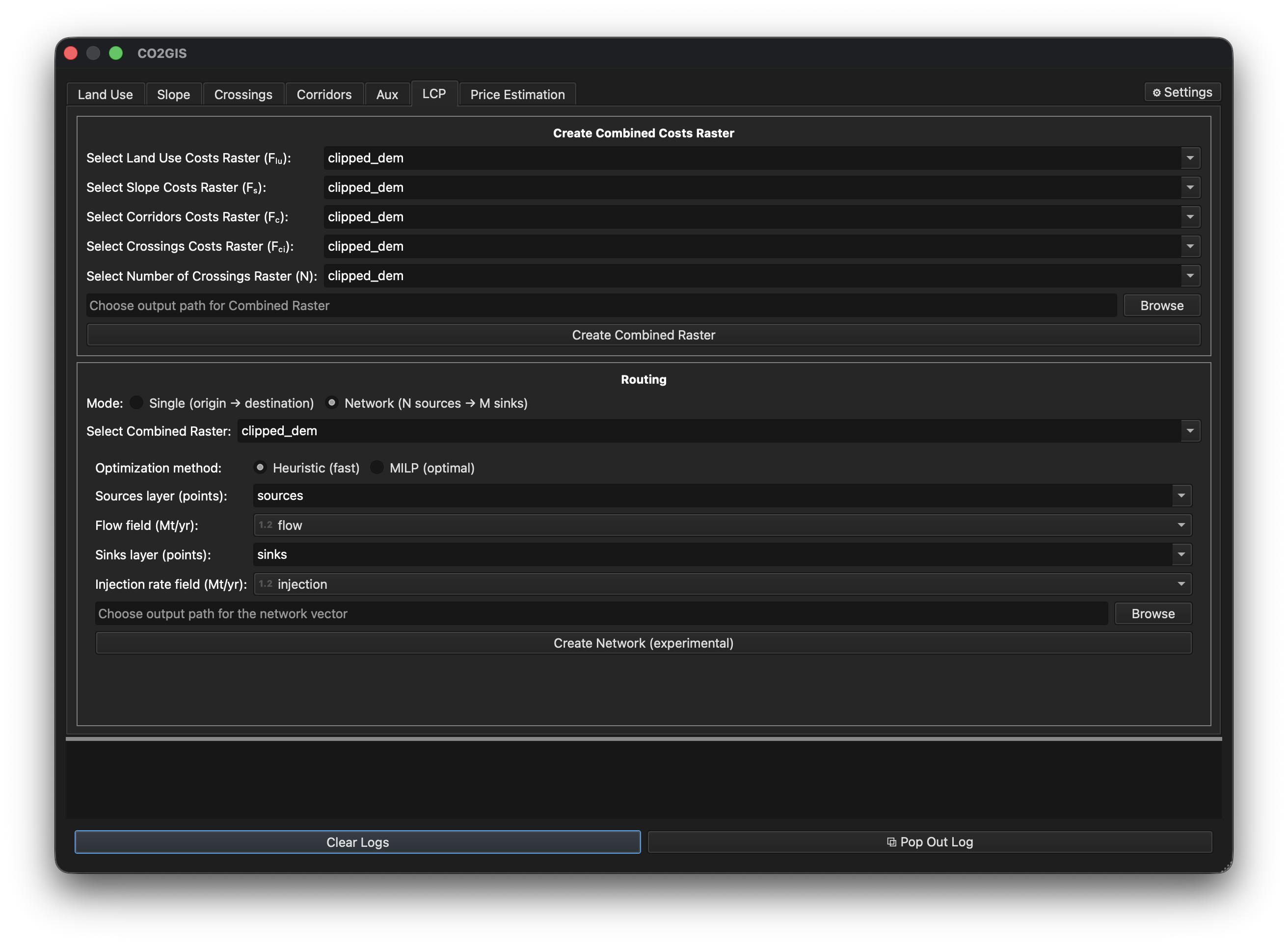
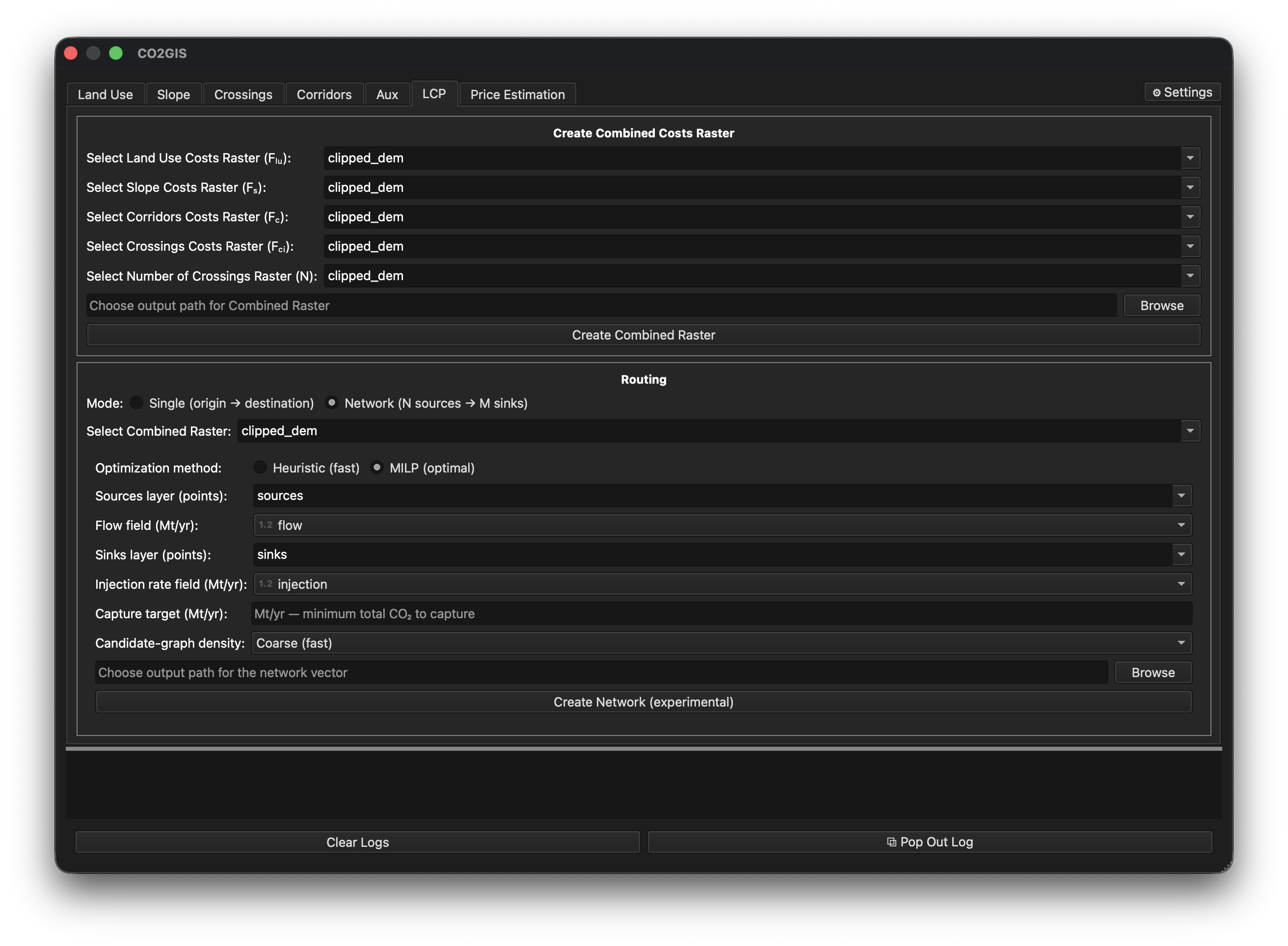
LCP tab in Network mode with Heuristic engine selected

MILP (optimal) — requires pulp and highspy installed in the QGIS Python environment:

pip install pulp highspy

If the solver is missing, the MILP radio is disabled and the tooltip tells you what to install. When available, two extra inputs appear:

Capture target (Mt/yr) — the minimum total CO₂ the network must move. The MILP selects the cheapest subset of sources that meets this target.
Candidate-graph density — how fine a junction grid the optimiser searches:

Preset	Speed	Accuracy
Coarse	fastest	rough
Medium (default)	balanced	good
Fine	slowest	closest to true optimum

Start with Coarse and refine if needed. The grid spacing is derived from your data’s extent automatically — no CRS-unit knowledge needed.

LCP tab in Network mode with MILP engine selected — shows Capture target and Candidate-graph density inputs

4. Run

Set an output path for the network GeoPackage and click Create Network (experimental). The log narrates progress:

Heuristic — each source tying into the network in turn.
MILP — candidate-graph size, solve status, and each drained link with its chosen pipe size.

5. Read the output

A network layer is loaded with one LineString per segment, with three fields:

Field	Meaning
`flow`	CO₂ flow through the segment (Mt/yr). A trunk carries the sum of the merged source flows.
`length`	Segment length in map units.
`junction`	1 if the segment starts at a junction (where flows merge); 0 otherwise.

Styling tip: graduate the line width by flow to see spurs thicken into trunks at the junctions — the visual signature of a shared-trunk network.

6. Price the network

Pricing is done in the Price Estimation tab, which also gains a Network mode when the experimental toggle is on:

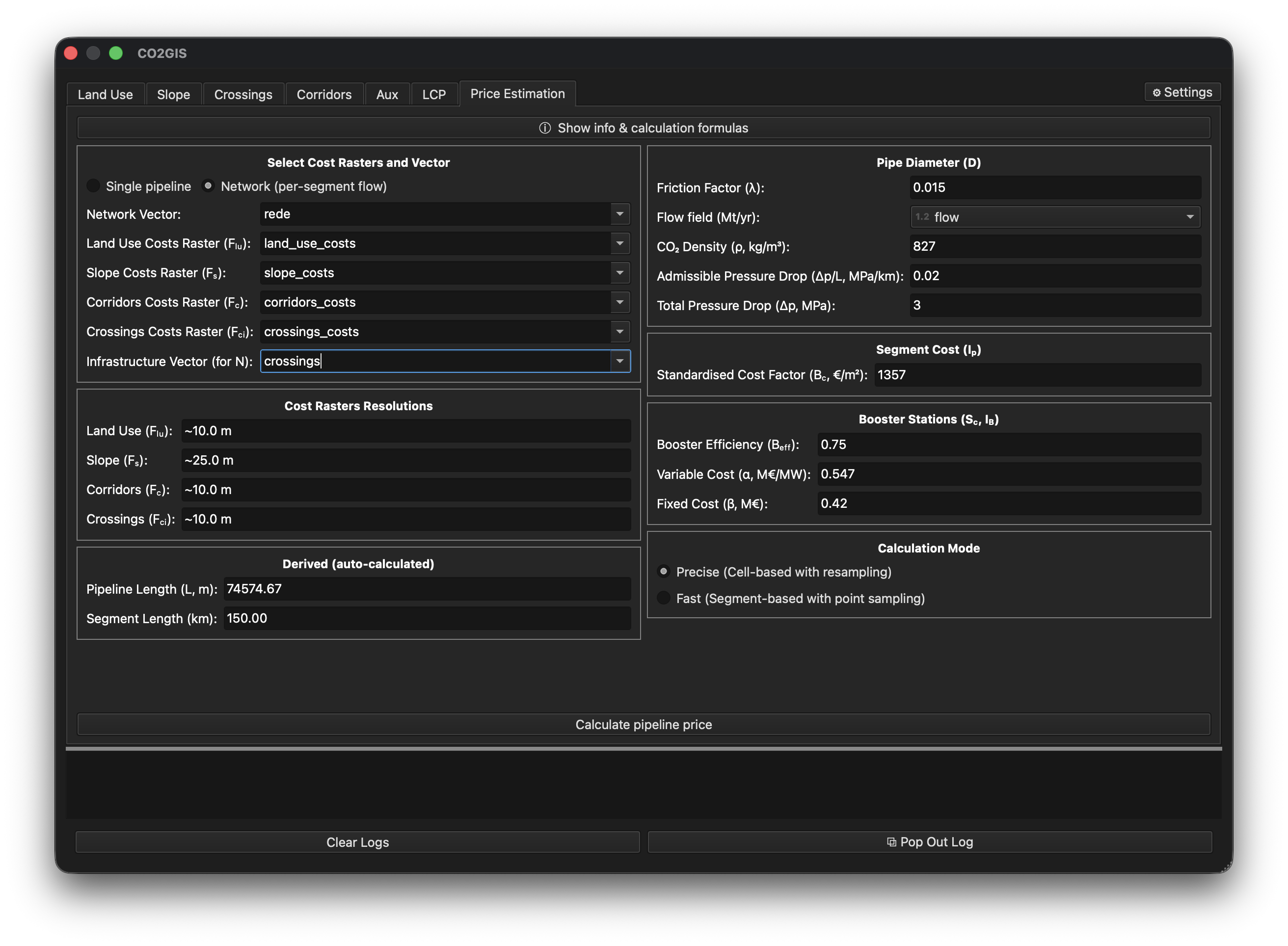
Price Estimation tab in Network mode — select the network vector and its flow field

Switch Price Estimation to Network mode.
Select the network.gpkg produced above and its flow field.
Run the estimate.

Each segment is sized for its own flow, split into pressure-budget segments with spacing boosters, and a junction booster is added where flows merge. The result is a total investment cost plus a per-pipe / per-junction breakdown.

See Network CAPEX for the pricing details.