The workflow
Price Estimation (CAPEX)
Estimate the route's capital cost from the cost rasters and flow parameters.
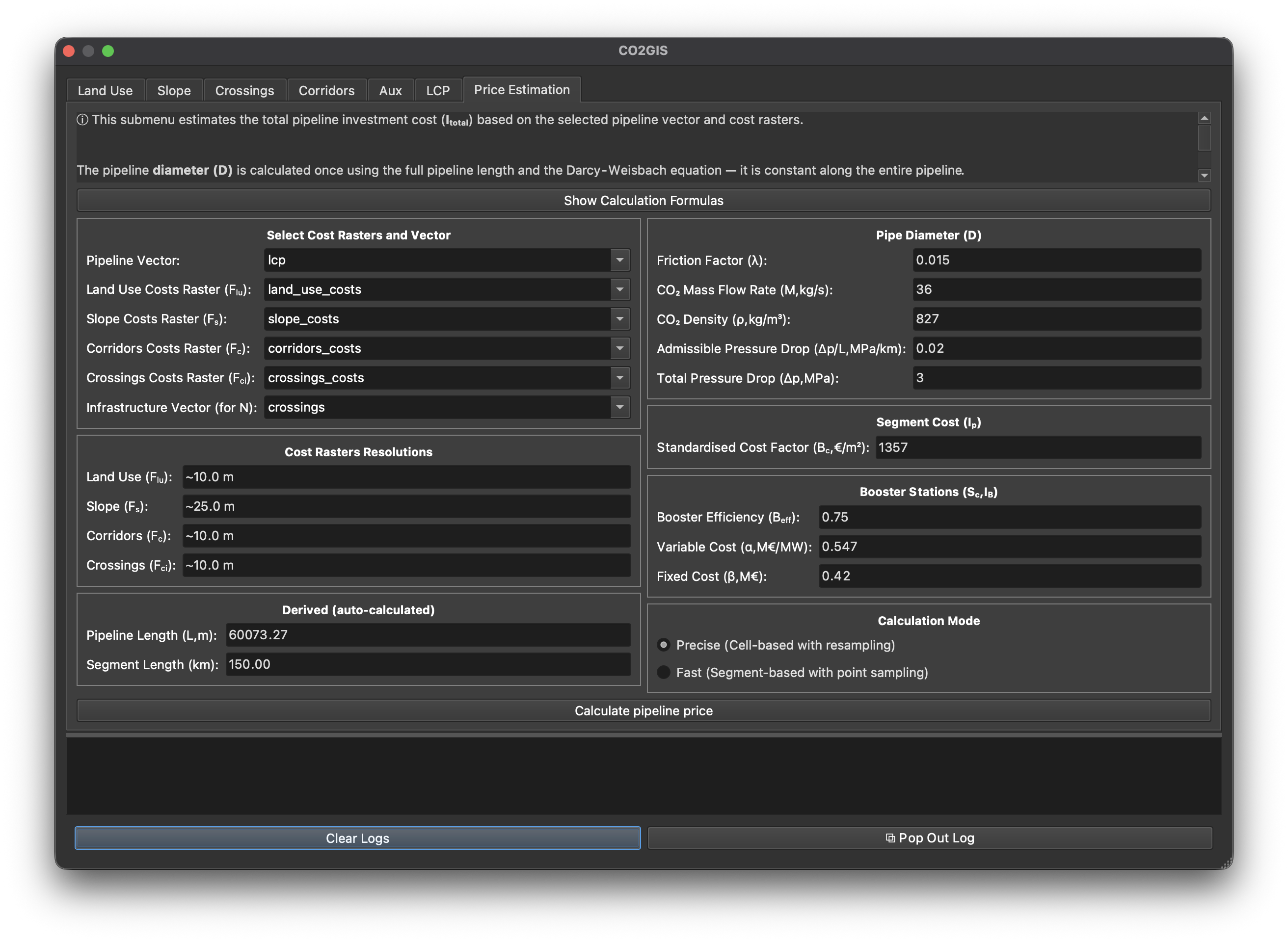
The Price Estimation tab estimates the route’s total CAPEX (I_total). It is split into two columns: the left column holds the data inputs (rasters and vectors), and the right column holds the equation parameters grouped by the formula each one feeds into.
Click Show Calculation Formulas to see all equations in a pop-up dialog. Results are written to the log at the bottom of the plugin.
Left column
Select Cost Rasters and Vector
| Field | What to select |
|---|---|
| Pipeline Vector | The route produced by the LCP tab |
| Land Use Costs Raster (F_lu) | Land-use cost surface |
| Slope Costs Raster (F_s) | Slope cost surface |
| Corridors Costs Raster (F_c) | Existing-corridor cost surface |
| Crossings Costs Raster (F_ci) | Road/rail crossing cost surface |
| Infrastructure Vector (for N) | Road/rail vector used to count crossings (N) |
A missing cost raster defaults to 1.0 (neutral multiplier). A missing infrastructure vector sets N = 1 for all cells, which keeps the F_ci term active without under-counting.
Cost Rasters Resolutions
Read-only fields auto-filled from each raster’s metadata. Shown so you can quickly verify the native cell size before choosing a resampling target in Precise mode.
Derived (auto-calculated)
| Field | How it is computed |
|---|---|
| Pipeline Length (L, m) | Total geometry length read from the selected pipeline vector |
| Segment Length (km) | Total Pressure Drop ÷ Admissible Pressure Drop — updates live as you edit those inputs |
Right column
Pipe Diameter (D)
The diameter is calculated once for the entire pipeline using the Darcy-Weisbach equation and stays constant along its full length. See Pipeline diameter for the formula.
| Input | Default | Meaning |
|---|---|---|
| Friction Factor (λ) | 0.015 | Darcy friction factor for CO₂ in steel pipe |
| CO₂ Mass Flow Rate (M, kg/s) | 1 | Design mass flow rate |
| CO₂ Density (ρ, kg/m³) | 827 | Supercritical CO₂ density |
| Admissible Pressure Drop (Δp/L, MPa/km) | 0.02 | Maximum allowable pressure loss per kilometre; also drives the Segment Length |
| Total Pressure Drop (Δp, MPa) | 3 | Maximum pressure loss one segment can sustain; also drives the Segment Length |
Segment Cost (I_p)
Each pipeline segment cost reuses the COMET cell costs weighted by the crossed cell lengths. See Segments & booster stations.
| Input | Default | Meaning |
|---|---|---|
| Standardised Cost Factor (B_c, €/m²) | 1357 | Base cost per metre squared of pipe cross-section; COMET default is in €₂₀₁₀ — replace with a current-year value to update prices |
Booster Stations (S_c, I_B)
Booster stations are placed between segments whenever the route exceeds one segment length. Their compressor power (S_c) and cost (I_B) depend on the three inputs below. See Segments & booster stations for the formulas.
| Input | Default | Meaning |
|---|---|---|
| Booster Efficiency (B_eff) | 0.75 | Compressor isentropic efficiency |
| Variable Cost (α, M€/MW) | 0.547 | Cost per MW of compressor capacity — scales with station size |
| Fixed Cost (β, M€) | 0.42 | Fixed installation cost per station, independent of size (civil, electrical, instrumentation) |
Default α and β are in M€₂₀₁₀ (COMET reference values). Replace with current figures to work in today’s prices.
Calculation Mode
Choose how cost factors are read along the route — see Precise vs fast mode for the full trade-off.
| Mode | How it works |
|---|---|
| Precise (default) | Resamples all rasters to a common grid; reads exact factor values and computes L_cell by geometric intersection for every cell the pipeline crosses |
| Fast | No resampling; samples 5 equally-spaced points along each vertex-to-vertex segment and takes the maximum — faster but slightly over-estimates cost |